pippy • pippy

Background

The aim of pippy is to make it easy for users to adopt a functional approach to their analysis with pipelines. Pipelines are defined using a reduced subset of R and, when run, use an intelligent approach to work planning and object caching. It was motivated by a desire to reduce the boilerplate I was writing with my R scripts and associated Makefiles. Whilst the goal is to be “good enough” for many pieces of analysis, by encouraging a functional approach, it remains easy to move to more advanced alternatives such as targets.

Scope

Goals:

🗸 Intelligent caching to reduce unnecessary execution.
🗸 Configuration files using a reduced subset of base R as their syntax.
🗸 Simple and efficient approach to managing multiple scenarios.

Out of scope:

🗴 HPC orchestration.
🗴 Automatic parallelisation of the pipeline.
🗴 Environment management.

The limitation is fundamental to pippy’s design. We make no attempt to handle changes across package or R versions and assume this environment is fixed. When packages used by pipelines are updated then pipelines should be rerun (likewise across R version updates).

A motivating example

The easiest way to get started with the package is to look at a template pipeline included within the package. create_skeleton_pipeline() can be used to set up a pipeline based on the mtcars data set and multiple scenarios.

library(pippy)
dir <- create_skeleton_pipeline(dir = tempfile())
od <- setwd(dir)

#> ✔ Template pipeline created in '/tmp/Rtmp8AuTWk/file2b675caf6a87'.

We now have the following in dir:

#> /tmp/Rtmp8AuTWk/file2b675caf6a87
#> ├── R
#> │   ├── load_dat.R
#> │   ├── plot_dat.R
#> │   └── wrangle_dat.R
#> ├── config.R
#> ├── data
#> │   └── mtcars.csv
#> └── pipeline.R

The pipeline we are going to run is described in pipeline.R:

pipeline.R

out <- run_pipeline(
    {
        raw   <- load_dat(CONFIG$in_csv)
        clean <- wrangle_dat(raw, CONFIG$rows)
        plot  <- plot_dat(clean, CONFIG$out_plot)
    },
    scenario = "production",
    scenario_default = "default")

run_pipeline() takes an expression where each assignment it contains represents a stage of the analysis. There are a few things to note about the expression syntax:

The left-hand-side (target) of each assignment must be uniquely named.
Function calls on the right-hand-side (rhs) must be defined in the function directory R or contained in the base R or stats namespaces.
The target names cannot match the names of functions in base R, or those contained in the function directory.
The order of assignments is not important as it is determined internally by the function.
Values from the configuration file, config.R, are accessed by the special CONFIG value (a list which can be subset using the $ symbol).

The last two entries relate to the configuration file:

scenario_default tells the function to parse the configuration file, looking for an entry called ‘default’. This is used as the base scenario.
scenario (in this case ‘production’ but could be multiple ones) specifies other values in the configuration file that are then layered on top of this (internally using modifyList()) to generate additional scenarios to run.

The configuration file

Configuration files are simply R scripts that are evaluated in a dedicated environment.

Scenarios are defined by named lists.

Within this environment we enable two special functions INFILE and OUTFILE:

INFILE() marks a file as an input. This ensures that run_pipeline() knows to keep a hash of the object and to monitor it for future changes when the pipeline is rerun.
OUTFILE() marks a file name as an output. This ensures that outputs from different scenarios (see later) do not overwrite one another (output files get saved in a scenario-dependent directory). It also ensures that output files are recreated if they are deleted.

In our example we have the following configuration file:

config.R

default <- list(
    in_csv   = INFILE("data/mtcars.csv"),
    out_plot = OUTFILE("plot.png"),
    rows     = 10
)

production <- list(
    rows = 32
)

Here in_csv points to our input data and out_plot to a png output file. The ‘production’ scenario will then be the same as the default but with the number of rows selected being 32, not 10.

This time the configuration file defines two scenarios, default, which subsets the data to 10 rows and production, which returns 32 rows.

The R directory

This is the directory where users define functions that represent stages of their analysis (e.g. cleaning data, modelling, plotting, …). Here we have:

R/load_dat.R

load_dat <- function(file) {
    stopifnot(file.exists(file))
    # Note: If function not in the base/stats namespace or function directory
    #       we must explictly namespace the call using `::`.
    utils::read.csv(file)
}

This file contains a single function which takes the filename of raw data as input before doing a little wrangling and returning the output. Note the comment about namespacing functions; anything not in the base/stats namespace or the function directory needs to be explicitly namespaced.

Next we have:

R/wrangle_dat.R

wrangle_dat <- function(dat, rows) {
    stopifnot(is.data.frame(dat), nrow(dat) >= rows, rows >= 0)
    head(dat, rows)
}

This function curtails the number of rows of data. Here we also make use of assertions in the function, checking that dat is a data frame and rows is between 0 and the number of rows in the data frame (inclusive). Assertions like these can be thought of unit tests for your analysis. Whilst here we have them at the start of the function to check inputs, they can be used anywhere in your function to ensure things are running as expected. If an assertion fails it will stop the pipeline running, bringing your attention to any issue at hand.

Finally there is

R/plot.R

plot_dat <- function(dat, outfile) {
    grDevices::png(outfile)
    plot(factor(dat$cyl), dat$mpg, xlab = "cyl", ylab = "mpg")
    grDevices::dev.off()
    # return name of where image is saved
    outfile
}

This function takes the manipulated data as input and creates a plot which is saved as a png. When saving output to disk, we recommend that the function returns the location where the file is saved for later use.

Putting it together

Running the pipeline we see the following

out <- run_pipeline(
    {
        raw <- load_dat(CONFIG$in_csv)
        clean <- wrangle_dat(raw, CONFIG$rows)
        plot <- plot_dat(clean, CONFIG$out_plot)
    },
    scenario = c("default", "production"),
    scenario_default = "default" # included here but note that this is
                                 # also the default value for the argument.
)

#>
#> ── Starting pipeline with `default` configuration ──────────────────────────────
#> ℹ Running function to generate object `raw`.
#> ℹ Saving `raw` to disk.
#> ℹ Running function to generate object `clean`.
#> ℹ Saving `clean` to disk.
#> ℹ Running function to generate object `plot`.
#> ℹ Saving `plot` to disk.
#>
#> ── Starting pipeline with `production` configuration ───────────────────────────
#> ℹ Loading object `raw` from disk cache.
#> ℹ Running function to generate object `clean`.
#> ℹ Saving `clean` to disk.
#> ℹ Running function to generate object `plot`.
#> ℹ Saving `plot` to disk.
#>
#> ── pipeline(s) finished ────────────────────────────────────────────────────────

We see above that the default scenario ran from scratch where as the production scenario was able to skip the first computation, loading the cached result from disk. This caching can also takes account of changes in functions within the function directory but does not attempt to handle changes in the underlying R version or packages you use (in essence, it assumes environment stability is managed elsewhere).

Each target output is saved within a named list associated with the relevant scenario.

str(out)
#> List of 2
#>  $ default   :List of 3
#>   ..$ clean:'data.frame':    10 obs. of  12 variables:
#>   .. ..$ car : chr [1:10] "Mazda RX4" "Mazda RX4 Wag" "Datsun 710" "Hornet 4 Drive" ...
#>   .. ..$ mpg : num [1:10] 21 21 22.8 21.4 18.7 18.1 14.3 24.4 22.8 19.2
#>   .. ..$ cyl : int [1:10] 6 6 4 6 8 6 8 4 4 6
#>   .. ..$ disp: num [1:10] 160 160 108 258 360 ...
#>   .. ..$ hp  : int [1:10] 110 110 93 110 175 105 245 62 95 123
#>   .. ..$ drat: num [1:10] 3.9 3.9 3.85 3.08 3.15 2.76 3.21 3.69 3.92 3.92
#>   .. ..$ wt  : num [1:10] 2.62 2.88 2.32 3.21 3.44 ...
#>   .. ..$ qsec: num [1:10] 16.5 17 18.6 19.4 17 ...
#>   .. ..$ vs  : int [1:10] 0 0 1 1 0 1 0 1 1 1
#>   .. ..$ am  : int [1:10] 1 1 1 0 0 0 0 0 0 0
#>   .. ..$ gear: int [1:10] 4 4 4 3 3 3 3 4 4 4
#>   .. ..$ carb: int [1:10] 4 4 1 1 2 1 4 2 2 4
#>   ..$ plot : chr "/tmp/Rtmp8AuTWk/file2b675caf6a87/output/default/plot.png"
#>   .. ..- attr(*, "OUTFILE")= logi TRUE
#>   ..$ raw  :'data.frame':    32 obs. of  12 variables:
#>   .. ..$ car : chr [1:32] "Mazda RX4" "Mazda RX4 Wag" "Datsun 710" "Hornet 4 Drive" ...
#>   .. ..$ mpg : num [1:32] 21 21 22.8 21.4 18.7 18.1 14.3 24.4 22.8 19.2 ...
#>   .. ..$ cyl : int [1:32] 6 6 4 6 8 6 8 4 4 6 ...
#>   .. ..$ disp: num [1:32] 160 160 108 258 360 ...
#>   .. ..$ hp  : int [1:32] 110 110 93 110 175 105 245 62 95 123 ...
#>   .. ..$ drat: num [1:32] 3.9 3.9 3.85 3.08 3.15 2.76 3.21 3.69 3.92 3.92 ...
#>   .. ..$ wt  : num [1:32] 2.62 2.88 2.32 3.21 3.44 ...
#>   .. ..$ qsec: num [1:32] 16.5 17 18.6 19.4 17 ...
#>   .. ..$ vs  : int [1:32] 0 0 1 1 0 1 0 1 1 1 ...
#>   .. ..$ am  : int [1:32] 1 1 1 0 0 0 0 0 0 0 ...
#>   .. ..$ gear: int [1:32] 4 4 4 3 3 3 3 4 4 4 ...
#>   .. ..$ carb: int [1:32] 4 4 1 1 2 1 4 2 2 4 ...
#>  $ production:List of 3
#>   ..$ clean:'data.frame':    32 obs. of  12 variables:
#>   .. ..$ car : chr [1:32] "Mazda RX4" "Mazda RX4 Wag" "Datsun 710" "Hornet 4 Drive" ...
#>   .. ..$ mpg : num [1:32] 21 21 22.8 21.4 18.7 18.1 14.3 24.4 22.8 19.2 ...
#>   .. ..$ cyl : int [1:32] 6 6 4 6 8 6 8 4 4 6 ...
#>   .. ..$ disp: num [1:32] 160 160 108 258 360 ...
#>   .. ..$ hp  : int [1:32] 110 110 93 110 175 105 245 62 95 123 ...
#>   .. ..$ drat: num [1:32] 3.9 3.9 3.85 3.08 3.15 2.76 3.21 3.69 3.92 3.92 ...
#>   .. ..$ wt  : num [1:32] 2.62 2.88 2.32 3.21 3.44 ...
#>   .. ..$ qsec: num [1:32] 16.5 17 18.6 19.4 17 ...
#>   .. ..$ vs  : int [1:32] 0 0 1 1 0 1 0 1 1 1 ...
#>   .. ..$ am  : int [1:32] 1 1 1 0 0 0 0 0 0 0 ...
#>   .. ..$ gear: int [1:32] 4 4 4 3 3 3 3 4 4 4 ...
#>   .. ..$ carb: int [1:32] 4 4 1 1 2 1 4 2 2 4 ...
#>   ..$ plot : chr "/tmp/Rtmp8AuTWk/file2b675caf6a87/output/production/plot.png"
#>   .. ..- attr(*, "OUTFILE")= logi TRUE
#>   ..$ raw  :'data.frame':    32 obs. of  12 variables:
#>   .. ..$ car : chr [1:32] "Mazda RX4" "Mazda RX4 Wag" "Datsun 710" "Hornet 4 Drive" ...
#>   .. ..$ mpg : num [1:32] 21 21 22.8 21.4 18.7 18.1 14.3 24.4 22.8 19.2 ...
#>   .. ..$ cyl : int [1:32] 6 6 4 6 8 6 8 4 4 6 ...
#>   .. ..$ disp: num [1:32] 160 160 108 258 360 ...
#>   .. ..$ hp  : int [1:32] 110 110 93 110 175 105 245 62 95 123 ...
#>   .. ..$ drat: num [1:32] 3.9 3.9 3.85 3.08 3.15 2.76 3.21 3.69 3.92 3.92 ...
#>   .. ..$ wt  : num [1:32] 2.62 2.88 2.32 3.21 3.44 ...
#>   .. ..$ qsec: num [1:32] 16.5 17 18.6 19.4 17 ...
#>   .. ..$ vs  : int [1:32] 0 0 1 1 0 1 0 1 1 1 ...
#>   .. ..$ am  : int [1:32] 1 1 1 0 0 0 0 0 0 0 ...
#>   .. ..$ gear: int [1:32] 4 4 4 3 3 3 3 4 4 4 ...
#>   .. ..$ carb: int [1:32] 4 4 1 1 2 1 4 2 2 4 ...
str(out$default$clean)
#> 'data.frame':    10 obs. of  12 variables:
#>  $ car : chr  "Mazda RX4" "Mazda RX4 Wag" "Datsun 710" "Hornet 4 Drive" ...
#>  $ mpg : num  21 21 22.8 21.4 18.7 18.1 14.3 24.4 22.8 19.2
#>  $ cyl : int  6 6 4 6 8 6 8 4 4 6
#>  $ disp: num  160 160 108 258 360 ...
#>  $ hp  : int  110 110 93 110 175 105 245 62 95 123
#>  $ drat: num  3.9 3.9 3.85 3.08 3.15 2.76 3.21 3.69 3.92 3.92
#>  $ wt  : num  2.62 2.88 2.32 3.21 3.44 ...
#>  $ qsec: num  16.5 17 18.6 19.4 17 ...
#>  $ vs  : int  0 0 1 1 0 1 0 1 1 1
#>  $ am  : int  1 1 1 0 0 0 0 0 0 0
#>  $ gear: int  4 4 4 3 3 3 3 4 4 4
#>  $ carb: int  4 4 1 1 2 1 4 2 2 4
str(out$production$clean)
#> 'data.frame':    32 obs. of  12 variables:
#>  $ car : chr  "Mazda RX4" "Mazda RX4 Wag" "Datsun 710" "Hornet 4 Drive" ...
#>  $ mpg : num  21 21 22.8 21.4 18.7 18.1 14.3 24.4 22.8 19.2 ...
#>  $ cyl : int  6 6 4 6 8 6 8 4 4 6 ...
#>  $ disp: num  160 160 108 258 360 ...
#>  $ hp  : int  110 110 93 110 175 105 245 62 95 123 ...
#>  $ drat: num  3.9 3.9 3.85 3.08 3.15 2.76 3.21 3.69 3.92 3.92 ...
#>  $ wt  : num  2.62 2.88 2.32 3.21 3.44 ...
#>  $ qsec: num  16.5 17 18.6 19.4 17 ...
#>  $ vs  : int  0 0 1 1 0 1 0 1 1 1 ...
#>  $ am  : int  1 1 1 0 0 0 0 0 0 0 ...
#>  $ gear: int  4 4 4 3 3 3 3 4 4 4 ...
#>  $ carb: int  4 4 1 1 2 1 4 2 2 4 ...
out$default$plot
#> [1] "/tmp/Rtmp8AuTWk/file2b675caf6a87/output/default/plot.png"
#> attr(,"OUTFILE")
#> [1] TRUE
out$production$plot
#> [1] "/tmp/Rtmp8AuTWk/file2b675caf6a87/output/production/plot.png"
#> attr(,"OUTFILE")
#> [1] TRUE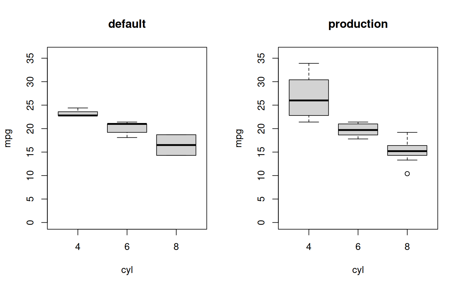

Two side by side box plots of cyl (x-axis) versus mpg (y-axis). The left-hand one represents the 'default' configuration, the right-hand, 'production'. There is a downward trend showing in mpg as cyl increases. — The resulting plots in the ‘output’ directory.

Changing things

Let’s assume that after cleaning our data we wanted to sample rows rather than take as is. Let’s add a new function to our R directory:

R/sample_clean.R

sample_clean <- function(clean) {
    clean[sample(nrow(clean), replace = TRUE), ]
}

cat(
    "sample_clean <- function(clean) clean[sample(nrow(clean), replace = TRUE), ]",
    file = file.path("R", "sample_clean.R")
)

Updating our pipeline accordingly, we now also set the seed

set.seed(1)
out <- run_pipeline(
    {
        raw     <- load_dat(CONFIG$in_csv)
        clean   <- wrangle_dat(raw, CONFIG$rows)
        samples <- sample_clean(clean)
        plot    <- plot_dat(samples, CONFIG$out_plot)
    },
    scenario = "production",
    scenario_default = "default"
)

#>
#> ── Starting pipeline with `default` configuration ──────────────────────────────
#> ℹ Running function to generate object `raw`.
#> ℹ Saving `raw` to disk.
#> ℹ Running function to generate object `clean`.
#> ℹ Saving `clean` to disk.
#> ℹ Running function to generate object `samples`.
#> ℹ Saving `samples` to disk.
#> ℹ Running function to generate object `plot`.
#> ℹ Saving `plot` to disk.
#>
#> ── Starting pipeline with `production` configuration ───────────────────────────
#> ℹ Loading object `raw` from disk cache.
#> ℹ Running function to generate object `clean`.
#> ℹ Saving `clean` to disk.
#> ℹ Running function to generate object `samples`.
#> ℹ Saving `samples` to disk.
#> ℹ Running function to generate object `plot`.
#> ℹ Saving `plot` to disk.
#>
#> ── Starting cleanup ────────────────────────────────────────────────────────────
#> ℹ Removing old objects that are no longer needed.
#>
#> ── pipeline(s) finished ────────────────────────────────────────────────────────

This time our caching ensured that once the samples were generated only the plotting function needed rerunning. Setting the seed ensures that we can load objects from the cache.

set.seed(1)
out <- run_pipeline(
    {
        raw     <- load_dat(CONFIG$in_csv)
        clean   <- wrangle_dat(raw, CONFIG$rows)
        samples <- sample_clean(clean)
        plot    <- plot_dat(samples, CONFIG$out_plot)
    },
    scenario = "production",
    scenario_default = "default"
)

#>
#> ── Starting pipeline with `default` configuration ──────────────────────────────
#> ℹ Loading object `raw` from disk cache.
#> ℹ Loading object `clean` from disk cache.
#> ℹ Loading object `samples` from disk cache.
#> ℹ Loading object `plot` from disk cache.
#>
#> ── Starting pipeline with `production` configuration ───────────────────────────
#> ℹ Loading object `raw` from disk cache.
#> ℹ Loading object `clean` from disk cache.
#> ℹ Loading object `samples` from disk cache.
#> ℹ Loading object `plot` from disk cache.
#>
#> ── pipeline(s) finished ────────────────────────────────────────────────────────

Once functionality introduces randomness, setting the seeds is needed to utilise the cache (even for non-random) output.

out <- run_pipeline(
    {
        raw     <- load_dat(CONFIG$in_csv)
        clean   <- wrangle_dat(raw, CONFIG$rows)
        samples <- sample_clean(clean)
        plot    <- plot_dat(samples, CONFIG$out_plot)
    },
    scenario = "production",
    scenario_default = "default"
)

#>
#> ── Starting pipeline with `default` configuration ──────────────────────────────
#> ℹ Running function to generate object `raw`.
#> ℹ Saving `raw` to disk.
#> ℹ Running function to generate object `clean`.
#> ℹ Saving `clean` to disk.
#> ℹ Running function to generate object `samples`.
#> ℹ Saving `samples` to disk.
#> ℹ Running function to generate object `plot`.
#> ℹ Saving `plot` to disk.
#>
#> ── Starting pipeline with `production` configuration ───────────────────────────
#> ℹ Loading object `raw` from disk cache.
#> ℹ Running function to generate object `clean`.
#> ℹ Saving `clean` to disk.
#> ℹ Running function to generate object `samples`.
#> ℹ Saving `samples` to disk.
#> ℹ Running function to generate object `plot`.
#> ℹ Saving `plot` to disk.
#>
#> ── Starting cleanup ────────────────────────────────────────────────────────────
#> ℹ Removing old objects that are no longer needed.
#>
#> ── pipeline(s) finished ────────────────────────────────────────────────────────

Loading objects from the cache

For large output, it can be beneficial not to return everything. To this end we provide a return argument to stop a running pipeline from returning it’s output. Output can then be accessed with load_pipeline_object:

out <- run_pipeline(
    {
        raw     <- load_dat(CONFIG$in_csv)
        clean   <- wrangle_dat(raw, CONFIG$rows)
        samples <- sample_clean(clean)
        plot    <- plot_dat(samples, CONFIG$out_plot)
    },
    scenario = "production",
    scenario_default = "default",
    return = FALSE
)

#>
#> ── Starting pipeline with `default` configuration ──────────────────────────────
#> ℹ Running function to generate object `raw`.
#> ℹ Saving `raw` to disk.
#> ℹ Running function to generate object `clean`.
#> ℹ Saving `clean` to disk.
#> ℹ Running function to generate object `samples`.
#> ℹ Saving `samples` to disk.
#> ℹ Running function to generate object `plot`.
#> ℹ Saving `plot` to disk.
#>
#> ── Starting pipeline with `production` configuration ───────────────────────────
#> ℹ Loading object `raw` from disk cache.
#> ℹ Running function to generate object `clean`.
#> ℹ Saving `clean` to disk.
#> ℹ Running function to generate object `samples`.
#> ℹ Saving `samples` to disk.
#> ℹ Running function to generate object `plot`.
#> ℹ Saving `plot` to disk.
#>
#> ── Starting cleanup ────────────────────────────────────────────────────────────
#> ℹ Removing old objects that are no longer needed.
#>
#> ── pipeline(s) finished ────────────────────────────────────────────────────────

str(out)
#>  NULL

By default all scenarios are returned:

load_pipeline_object("clean")

#> $default
#> $default$clean
#>                  car  mpg cyl  disp  hp drat    wt  qsec vs am gear carb
#> 1          Mazda RX4 21.0   6 160.0 110 3.90 2.620 16.46  0  1    4    4
#> 2      Mazda RX4 Wag 21.0   6 160.0 110 3.90 2.875 17.02  0  1    4    4
#> 3         Datsun 710 22.8   4 108.0  93 3.85 2.320 18.61  1  1    4    1
#> 4     Hornet 4 Drive 21.4   6 258.0 110 3.08 3.215 19.44  1  0    3    1
#> 5  Hornet Sportabout 18.7   8 360.0 175 3.15 3.440 17.02  0  0    3    2
#> 6            Valiant 18.1   6 225.0 105 2.76 3.460 20.22  1  0    3    1
#> 7         Duster 360 14.3   8 360.0 245 3.21 3.570 15.84  0  0    3    4
#> 8          Merc 240D 24.4   4 146.7  62 3.69 3.190 20.00  1  0    4    2
#> 9           Merc 230 22.8   4 140.8  95 3.92 3.150 22.90  1  0    4    2
#> 10          Merc 280 19.2   6 167.6 123 3.92 3.440 18.30  1  0    4    4
#>
#>
#> $production
#> $production$clean
#>                    car  mpg cyl  disp  hp drat    wt  qsec vs am gear carb
#> 1            Mazda RX4 21.0   6 160.0 110 3.90 2.620 16.46  0  1    4    4
#> 2        Mazda RX4 Wag 21.0   6 160.0 110 3.90 2.875 17.02  0  1    4    4
#> 3           Datsun 710 22.8   4 108.0  93 3.85 2.320 18.61  1  1    4    1
#> 4       Hornet 4 Drive 21.4   6 258.0 110 3.08 3.215 19.44  1  0    3    1
#> 5    Hornet Sportabout 18.7   8 360.0 175 3.15 3.440 17.02  0  0    3    2
#> 6              Valiant 18.1   6 225.0 105 2.76 3.460 20.22  1  0    3    1
#> 7           Duster 360 14.3   8 360.0 245 3.21 3.570 15.84  0  0    3    4
#> 8            Merc 240D 24.4   4 146.7  62 3.69 3.190 20.00  1  0    4    2
#> 9             Merc 230 22.8   4 140.8  95 3.92 3.150 22.90  1  0    4    2
#> 10            Merc 280 19.2   6 167.6 123 3.92 3.440 18.30  1  0    4    4
#> 11           Merc 280C 17.8   6 167.6 123 3.92 3.440 18.90  1  0    4    4
#> 12          Merc 450SE 16.4   8 275.8 180 3.07 4.070 17.40  0  0    3    3
#> 13          Merc 450SL 17.3   8 275.8 180 3.07 3.730 17.60  0  0    3    3
#> 14         Merc 450SLC 15.2   8 275.8 180 3.07 3.780 18.00  0  0    3    3
#> 15  Cadillac Fleetwood 10.4   8 472.0 205 2.93 5.250 17.98  0  0    3    4
#> 16 Lincoln Continental 10.4   8 460.0 215 3.00 5.424 17.82  0  0    3    4
#> 17   Chrysler Imperial 14.7   8 440.0 230 3.23 5.345 17.42  0  0    3    4
#> 18            Fiat 128 32.4   4  78.7  66 4.08 2.200 19.47  1  1    4    1
#> 19         Honda Civic 30.4   4  75.7  52 4.93 1.615 18.52  1  1    4    2
#> 20      Toyota Corolla 33.9   4  71.1  65 4.22 1.835 19.90  1  1    4    1
#> 21       Toyota Corona 21.5   4 120.1  97 3.70 2.465 20.01  1  0    3    1
#> 22    Dodge Challenger 15.5   8 318.0 150 2.76 3.520 16.87  0  0    3    2
#> 23         AMC Javelin 15.2   8 304.0 150 3.15 3.435 17.30  0  0    3    2
#> 24          Camaro Z28 13.3   8 350.0 245 3.73 3.840 15.41  0  0    3    4
#> 25    Pontiac Firebird 19.2   8 400.0 175 3.08 3.845 17.05  0  0    3    2
#> 26           Fiat X1-9 27.3   4  79.0  66 4.08 1.935 18.90  1  1    4    1
#> 27       Porsche 914-2 26.0   4 120.3  91 4.43 2.140 16.70  0  1    5    2
#> 28        Lotus Europa 30.4   4  95.1 113 3.77 1.513 16.90  1  1    5    2
#> 29      Ford Pantera L 15.8   8 351.0 264 4.22 3.170 14.50  0  1    5    4
#> 30        Ferrari Dino 19.7   6 145.0 175 3.62 2.770 15.50  0  1    5    6
#> 31       Maserati Bora 15.0   8 301.0 335 3.54 3.570 14.60  0  1    5    8
#> 32          Volvo 142E 21.4   4 121.0 109 4.11 2.780 18.60  1  1    4    2

We can restrict scenarios if we wish:

load_pipeline_object("clean", scenario = "default")

#> $default
#> $default$clean
#>                  car  mpg cyl  disp  hp drat    wt  qsec vs am gear carb
#> 1          Mazda RX4 21.0   6 160.0 110 3.90 2.620 16.46  0  1    4    4
#> 2      Mazda RX4 Wag 21.0   6 160.0 110 3.90 2.875 17.02  0  1    4    4
#> 3         Datsun 710 22.8   4 108.0  93 3.85 2.320 18.61  1  1    4    1
#> 4     Hornet 4 Drive 21.4   6 258.0 110 3.08 3.215 19.44  1  0    3    1
#> 5  Hornet Sportabout 18.7   8 360.0 175 3.15 3.440 17.02  0  0    3    2
#> 6            Valiant 18.1   6 225.0 105 2.76 3.460 20.22  1  0    3    1
#> 7         Duster 360 14.3   8 360.0 245 3.21 3.570 15.84  0  0    3    4
#> 8          Merc 240D 24.4   4 146.7  62 3.69 3.190 20.00  1  0    4    2
#> 9           Merc 230 22.8   4 140.8  95 3.92 3.150 22.90  1  0    4    2
#> 10          Merc 280 19.2   6 167.6 123 3.92 3.440 18.30  1  0    4    4

Finally we go back to our original directory

setwd(od)

Caveats

There are two important things to be aware of when using pippy:

We utilise R’s rds format for caching objects to disk. This means that functions should only return objects that are serialisable and unserialisable by that format.
We only hash functions defined by the user in the R/ directory, not those of underlying package dependencies. Updating packages or R can potentially invalidate the cache so it is the users responsibility to maintain a consistent environment, or force a rerun of the pipeline where necessary.